12 Pharmacaldynamic analysis

12.1 Variance covariance in repeated measures

Study deisgn: before and after Measure the same outcome before and after intervention. Interested in the change before and after the intervention within the same subject. We have \[Var(Y_{i2}- Y_{i1}) = Var(Y_{i1}) + Var(Y_{i2})- Cov(Y_{i1}, Y_{i2}) \\ = \sigma_1^2 +\sigma_2^2- 2\sigma_{12}\\ = \sigma_1^2 +\sigma_2^2- 2 \rho_{12} \sigma_1 \sigma_2\]

Comparing to the measurement between two independent subjects, we have \(\sigma_{12} =0\), which reduce the the variance \(Y_{i2}- Y_{i1}\) to \(\sigma_1^2 +\sigma_2^2\)

Assuming the vriance of response is constant across time. We have \(\sigma_1^2 =\sigma_2^2 = \sigma^2\), which reduce the within subject variance into \(2 \sigma^2(1-\rho)\)

This property gives us the ratio of within-subject/ between-subject variance: \(\frac{within-subject}{between-subject} = 1- \rho\)

12.2 Hierarchical modeling

12.2.1 GEE vs. GLMM

Generalized estimating equations(GEE) Generalized Linear Mixed Model (GLMM)

library(tidyr)
data(world_bank_pop)
pop2 <- world_bank_pop %>%
  pivot_longer(`2000`:`2017`, names_to = "year", values_to = "value") %>%
  dplyr::filter(
    indicator == "SP.POP.TOTL",
    year <= 2005
  )
dim(pop2)

## [1] 1584    4

table(world_bank_pop$indicator)

## 
## SP.POP.GROW SP.POP.TOTL SP.URB.GROW SP.URB.TOTL 
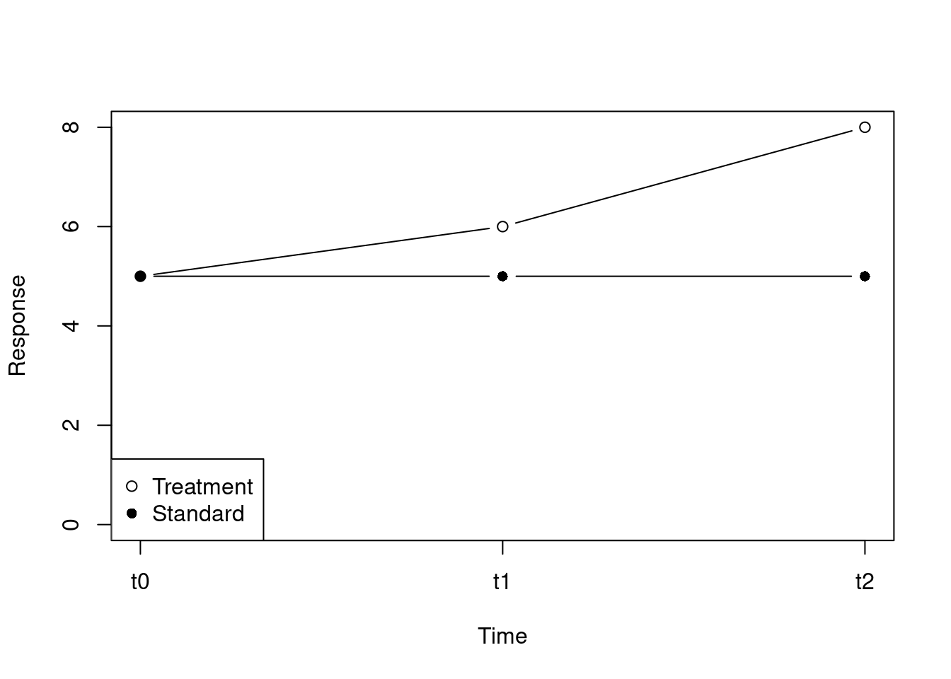
##         264         264         264         264

\[Y_{ij} = \beta_0+ \beta_1 Group + \beta_2 Time + \beta_3 Group \times time + \epsilon_{ij}\] i - subject; j - time points

Group	Time	coeff
reference	T0	\(\beta_0\)
treatment	T0	\(\beta_0 + \beta_1\)
reference	T1	\(\beta_0 + \beta_2\)
treatment	T1	\(\beta_0 + \beta_2 + \beta_3\)