10 Power and sample size

10.3.1 1. Agreement between two measurements

assess the agreement of two measurements

10.3.1.1 Inter-class correlation coefficient

Pearson correlation
Spearman correlation

\[ \frac{\sum_i\rho(G_{j}(Rseq), G_{j}(nano)))}{n_i} \]

i - number of genes
j - number of subjects

Need to visually examine if there exist ceiling and flooring effect between two measurements.

10.3.1.2 Intraclass Correlation Coefficient (ICC)

Generally speaking, the ICC determines the reliability of ratings by comparing the variability of different ratings of the same individuals to the total variation across all ratings and all individuals.

A high ICC (close to 1) indicates high similarity between values from the same group.
A low ICC (ICC close to zero) means that values from the same group are not similar.

The sample size is calculated based on following parameter:

ICC0 - ICC of null hypothesis (e.g. 0 no agreement or a value based on previous observations)
ICC - hypothetical ICC
alpha at 0.05
k = 2 (number of raters: nanostring vs. RNAseq)
two tails

Example calibration between RNAseq and nanostring measurements

library(ICC.Sample.Size)
library(tidyr)
library(kableExtra)
library(dplyr)

sample <- rep(c("RNAseq", "nanostring"), 3)
genes <- matrix(rnorm(30), ncol = 6)
rownames(genes) <- paste0("gene", c(1:5))
colnames(genes) <- sample
kable(genes, digits = 2) %>%
  add_header_above(c("", "ID1" = 2, "ID2" = 2, "ID3" = 2))

	ID1		ID2		ID3
	RNAseq	nanostring	RNAseq	nanostring	RNAseq	nanostring
gene1	-0.69	-1.46	-0.23	-0.52	0.97	1.04
gene2	-1.22	1.06	-0.03	-0.35	-1.23	-0.32
gene3	-1.07	-0.14	0.82	1.65	-0.94	0.49
gene4	-0.80	2.22	-0.49	0.18	-0.15	-0.66
gene5	-1.17	-0.66	-0.99	0.84	0.41	-1.31

Statistical power at 80%, single tail

k2a005p08 <- calculateIccSampleSize(by = "both", tails = 1)
table_n <- k2a005p08[[2]]

knitr::kable(table_n,
caption = "Table of sample size (N) given null and alterative hythosis of ICC.") %>%
  column_spec(2:12, color = ifelse(rownames(table_n) > 0.5, "red", 1)) %>%
  add_header_above(c("", "ICC0" = 20)) %>%
  pack_rows("ICC", 1, 20)

Table 10.1: Table of sample size (N) given null and alterative hythosis of ICC.
	ICC0
	0	0.05	0.1	0.15	0.2	0.25	0.3	0.35	0.4	0.45	0.5	0.55	0.6	0.65	0.7	0.75	0.8	0.85	0.9	0.95
ICC
0	Inf	2470	616	272	152	96	66	48	36	28	22	18	14	12	10	8	7	5	4	3
0.05	2470	Inf	2446	606	267	148	93	64	46	34	26	21	16	13	11	9	7	6	5	3
0.1	616	2446	Inf	2397	591	259	143	89	61	43	32	25	19	15	12	10	8	6	5	4
0.15	272	606	2397	Inf	2324	570	248	136	85	57	40	30	23	17	14	11	8	7	5	4
0.2	152	267	591	2324	Inf	2229	544	235	128	79	53	37	27	20	15	12	9	7	5	4
0.25	96	148	259	570	2229	Inf	2113	512	220	119	73	48	34	24	18	14	10	8	6	4
0.3	66	93	143	248	544	2113	Inf	1978	476	203	109	66	44	30	21	16	11	8	6	4
0.35	48	64	89	136	235	512	1978	Inf	1826	436	184	98	59	38	26	18	13	9	7	4
0.4	36	46	61	85	128	220	476	1826	Inf	1660	393	165	87	51	33	22	15	10	7	5
0.45	28	34	43	57	79	119	203	436	1660	Inf	1483	347	144	75	44	27	18	12	8	5
0.5	22	26	32	40	53	73	109	184	393	1483	Inf	1297	300	123	63	36	22	14	9	5
0.55	18	21	25	30	37	48	66	98	165	347	1297	Inf	1108	253	101	51	28	17	10	6
0.6	14	16	19	23	27	34	44	59	87	144	300	1108	Inf	918	205	80	39	21	12	6
0.65	12	13	15	17	20	24	30	38	51	75	123	253	918	Inf	732	160	61	28	14	7
0.7	10	11	12	14	15	18	21	26	33	44	63	101	205	732	Inf	555	117	42	18	8
0.75	8	9	10	11	12	14	16	18	22	27	36	51	80	160	555	Inf	393	79	26	10
0.8	7	7	8	8	9	10	11	13	15	18	22	28	39	61	117	393	Inf	251	46	13
0.85	5	6	6	7	7	8	8	9	10	12	14	17	21	28	42	79	251	Inf	134	20
0.9	4	5	5	5	5	6	6	7	7	8	9	10	12	14	18	26	46	134	Inf	49
0.95	3	3	4	4	4	4	4	4	5	5	5	6	6	7	8	10	13	20	49	Inf

10.3.2 2. Sample size for calibrations

10.3.2.1 The calibration function

The goal is to associate a test value (e.g. RNAseq) to a reference value (e.g. nanostring) via a calibration function. We collect N samples of paired measured: \(\{(X_i, Y_i), i = 1... N\}\), where \[ X_i = \tilde{X_i} + \epsilon_i^x \\ Y_i = \tilde{Y_i} + \epsilon_i^y\\ \tilde{Y_i} = f_0(\tilde{X_i}) +e_i \] where \(\epsilon_i^x ,\epsilon_i^y, e_i\) are zero mean errors with variance \(\sigma_i^{x2}, \sigma_i^{y2}, \sigma_0^2\)

In simple calibration function, we assume a linear function: \(f_0(x) = \beta_0+\beta_1X\). We want to estimage \(\beta_0, \beta_1\) to solve the calibration function.

Some considerations for calibration function:

the variance of the measurement error often depends on the underlying level.
standard deviation for the measurement error is proportional to the underlying value
the CV (SD/mean) of themeasurement error is approximately a constant

therefore the estimate of variance, assuming: \[ \sigma_i^x = CV_x \times \tilde{X} \\ \sigma_i^y = CV_x \times \tilde{Y} \\ \]

For estimating parameters in calibration function see the reference paper for different senarios.

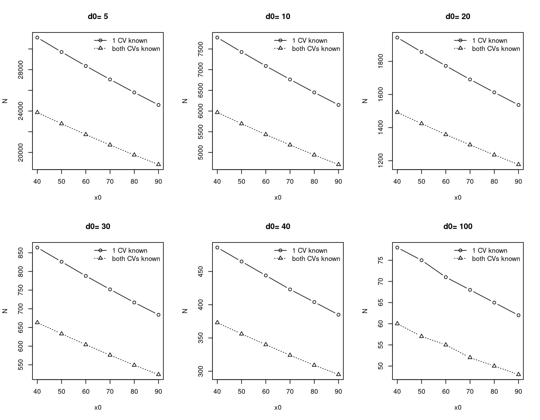
10.3.2.1.1 Sample size calculation for calibration

\[ N = max_{k=1..K}\bigg\{\frac{(2Z_{1-\alpha})^2\times \sigma^2(x_k)}{\delta_k^2}\bigg\}\\ \sigma^2(x_k) =(1, x_k)\sum\bigg(1, x_k\bigg) \]

\(\sum\) is variance, co-variance matrix for estimated intercept and slope of the calibration function. \(\delta_k, k = 1...K\) precision levels.

Parameters to consider before calculation:

x0: x value plan to calibrate with estimated calibration equation (e.g. \(\beta_0=0, \beta_1=1\), and this never happens in reality)
d0: 95% CI of calibrated x value
x: emperical observation of targeted distribution (e.g. mRNA levels from RNA seq or from nanostring)
CVx: coefficient variation of measurement X (e.g. nanostring), assume to be constant
CVy: coefficient variation of measurement Y (e.g. RNAseq), assume to be constant

10.3.2.2 Sample size calculation examples

CVx= CVy = 0.2

x0 <- c(40, 50, 60, 70, 80, 90)
d0 <- c(5, 10, 20, 30, 40, 100)

calc_samplesize <- function(x0, d0, x =seq(5, 1000, length = 1000), CVx =0.2, CVy=0.2) {
  CVcalibration::samplesize(x0, d0,
    x = x, # assuming RNAseq raw count data
    CVx = CVx, CVy = CVy
  )
}
par(mfrow = c(2, 3))
lapply(d0, function(d) {
  rst <- sapply(x0, function(x) calc_samplesize(x0 = x, d0 = d))
  tab <- do.call("rbind", rst)
  # rownames(tab) <- x0
  ymin <- min(tab)
  ymax <- max(tab)
  plot(x0, tab[, 1],
    type = "b",
    ylim = c(ymin, ymax),
    ylab = "N",
    main = paste("d0=", d)
  )
  lines(x0, tab[, 3], lty = 3, type = "b", pch = 2)
  legend("topright", c("1 CV known", "both CVs known"),
    bty = "n",
    lty = c(1, 3), pch = c(1, 2)
  )
  return(NULL)
})

10.3.3 Choosing samples range

There are two important considerations for choosing sampling methods: (i) the selected Xi values should cover the entire region of interest and (ii) the particular sampling scheme should help us to obtain an accurate estimate for the calibration function. There are several obvious choices:

randomly sampling from the stored samples (sample more from important regaions, but less accurate)

uniformly sampling from the given interval of interest (more accurate, less samples from important regions to investigate linear assumption) ;

a hybrid of the aforementioned two sampling methods (balance between above two):

dividing the range of interest into intervals using the quantiles of the observed samples

uniformly sampling equal number of Xi’s from each of the subintervals.

par(mfrow = c(1, 3))
set.seed(789)
x <- rnorm(500, 2)
x1 <- runif(500, -1, 5)
qt <- quantile(x)
x2 <- c(runif(100,qt[1], qt[2]), runif(100, qt[2], qt[3]), runif(100, qt[3], qt[4]), runif(100,qt[4], qt[5]))
hist(x, breaks =30, main ="random sampling")
hist(x1, breaks = 30, main ="uniform sampling")
hist(x2, breaks = 30, main = "hybrid sampling")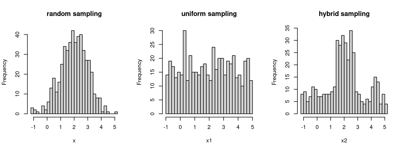

10.3.4 Estimating coefficient variation (CV) within the same measures

repeated measures in the same sample to obtain the estimation of CV in both techonologies

10.3.4.1 Consideration for prediction precision

Calibration can be viewed as a prediction model. Without any error measurement and assuming constant error variance, a linear model can be used: \[Y_i = a\beta X_i +b + \epsilon\]

Uncertainy will be considered when translating the cut-off from RNAseq data to Nanostring. It boils down to estimate with prediction the residual variance. When a sample of size \(n\) is drawn from a normal distribution, a \(1-\alpha\) CI of the unknown population variance is given by \[\frac{n-1}{\chi^2_{1-\alpha/2, n-1}}s^2 < \sigma^2 < \frac{n-1}{\chi^2_{\alpha/2, n-1}}s^2\] The fold change between the bounds (multiplicative margin of error) can be used as a precision proxy [4].

Formula can be adapted with \(p\) parameters [5]. Non linear relationship can be considered with a restricted cubic splines and k knots (k-1 parameters) We assume that k = 3f:

dat <- data.frame(
  MMOE = c(1.1, 1.2),
  linear = c(235, 71),
  non_linear = c(238, 74)
)

knitr::kable(dat)

MMOE	linear	non_linear
1.1	235	238
1.2	71	74

10.3.5 Final consideration for sample size

The sample size consideration should serve the purpose of analysis, which in our case is calibraion and agreement test. These two objectives might render different numbers. In order to gurantee the quality of prelminary analysis, we should take the max{N1, N2, N3}.

10.3.6 Reference

[1]T. K. Koo and M. Y. Li, “A Guideline of Selecting and Reporting Intraclass Correlation Coefficients for Reliability Research”, Journal of Chiropractic Medicine, vol. 15, no. 2, pp. 155-163, Jun. 2016, doi: 10.1016/j.jcm.2016.02.012.

[2]S. D. Walter, M. Eliasziw, and A. Donner, “Sample size and optimal designs for reliability studies”, Statistics in Medicine, vol. 17, no. 1, pp. 101–110, 1998, doi: 10.1002/(SICI)1097-0258(19980115)17:1<101::AID-SIM727>3.0.CO;2-E.

[3] L. Tian, R. A. Durazo-Arvizu, G. Myers, S. Brooks, K. Sarafin, and C. T. Sempos, “The estimation of calibration equations for variables with heteroscedastic measurement errors,” Statistics in Medicine, vol. 33, no. 25, pp. 4420-4436, 2014, doi: 10.1002/sim.6235.

[4]F. E. Harrell Jr., “Regression Modeling Strategies”. Springer International Publishing, 2016

[5]R. D. Riley, J. Ensor, K. I. E. Snell, et al. “Calculating the sample size required for developing a clinical prediction model”. BMJ. 2020